RF Planning – Standard Propagation Model Tuning in Atoll
Propagation Model
A propagation model provides an mathematical Equation for Calculating the Path Loss between the Transmitter and Receiver.
Models Types
- Physical models
- Physical models of path loss make use of physical radio waves principles such as free space transmission, reflection or diffraction.
- Empirical models
- Empirical models use measurement data to model a path loss equation. Examples of empirical propagation models include the ITU-R and the Hata models. Empirical models use what are known as predictors or specifies in general statistical modelling theory.
Standard Propagation Model
To get an accurate model for propagation losses is a big deal when planning a mobile radio network. The Standard Propagation Model (SPM), is based on empirical formulas and a set of parameters.
When Atoll RF planning tool is installed, the SPM parameters are set to their default values. However, they can be adjusted to tune the propagation model according to actual propagation conditions using Calibration or Model Tuning Procedure. This calibration process of the Standard Propagation Model facilitates improving the prediction reliability.
SPM formula
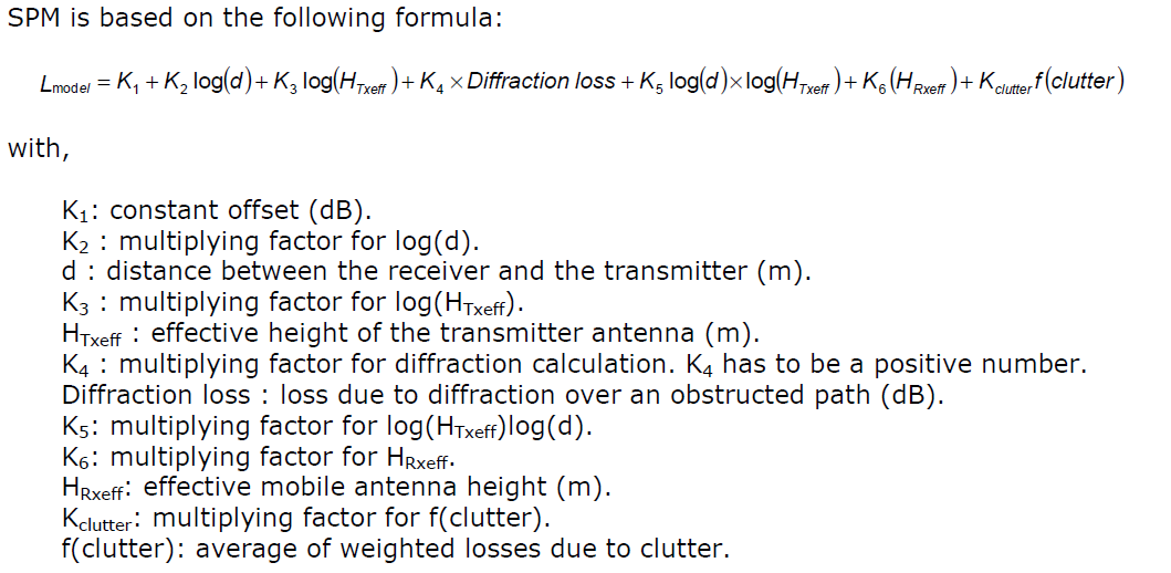
SPM is based on the following formula:
Action before Model Tuning
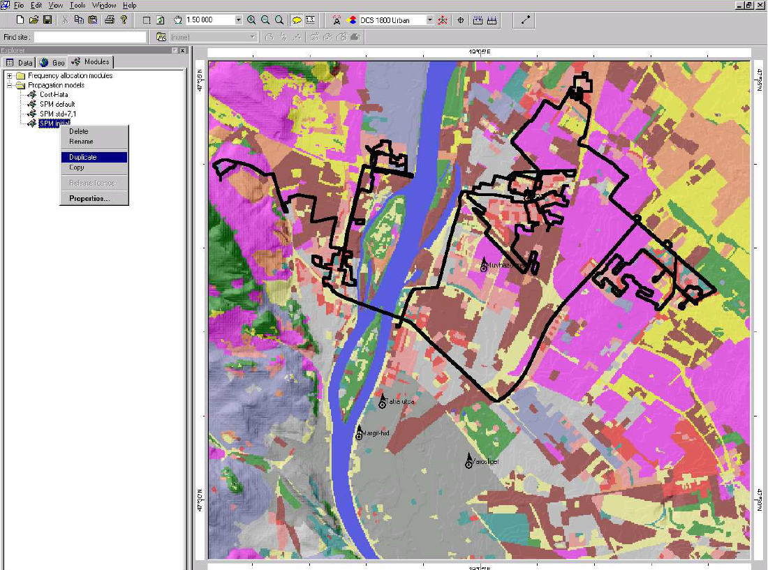
- Data validation: A quick data validation is to import the measurement files and a set of vector files that represent roads in Atoll, in order to check that the data correspond. Check that the measurement path starts and/or ends approximately at base station location. If possible check some pictures from base station neighbourhood to check that no close obstacle. If an obstacle is present in one direction, it is possible to filter the measurement data according to the orientation by fixing a negative and a positive angle for which the data will be taken into account.
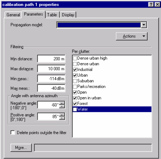
- Signal strength filter : The model tuning aims to produce an accurate model that will represent the propagation within the validity region of the model itself. For this reason, the model’s own constraints with respect to signal levels need to be taken into account. There are limitations in the measurement equipment with dynamic range capability, which also need to be taken into account.
Generally, signals above –40dBm are filtered out as they would be inaccurate due to receiver overload. For the minimum signal filtering, the sensitivity of the receiver and the tolerance have to be considered. So, signals below ‘receiver sensitivity + target standard deviation’ have to be filtered out to avoid the effect of noise saturation in the statistical results. - Distance filter: Measurement data at a distance less than 200m from the base station are discarded because these points are too close from the station to properly represent the propagation
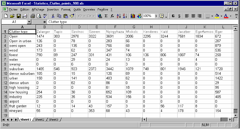
in the whole area. A common limit for the maximum distance is 10km. - Points Density Filter: Another filtering can be done according to the project related to the clutter classes. If only a few measurement paths contain a specific clutter class or only a few points are located in this class, then this clutter class can be filtered out. Keeping this class can, in fact, generate some bad statistical results or affect the model tuning incorrectly. For example, in the following case, the water class can be filtered out. This class would influence the prediction only in areas with large surfaces of water. Number of points per clutter class – measurement.
Model Tuning Steps
Step#1 Your model has the initial parameters necessary to start the tuning. It is advised to duplicate this modified model as it is rare to get a good calibration in the first attempt.
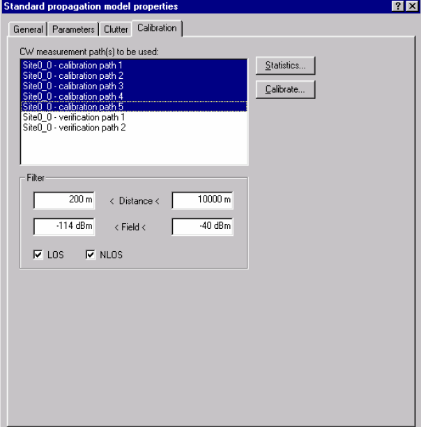
Step#2 The filters about the field and the distance are defined and applied in the measurement
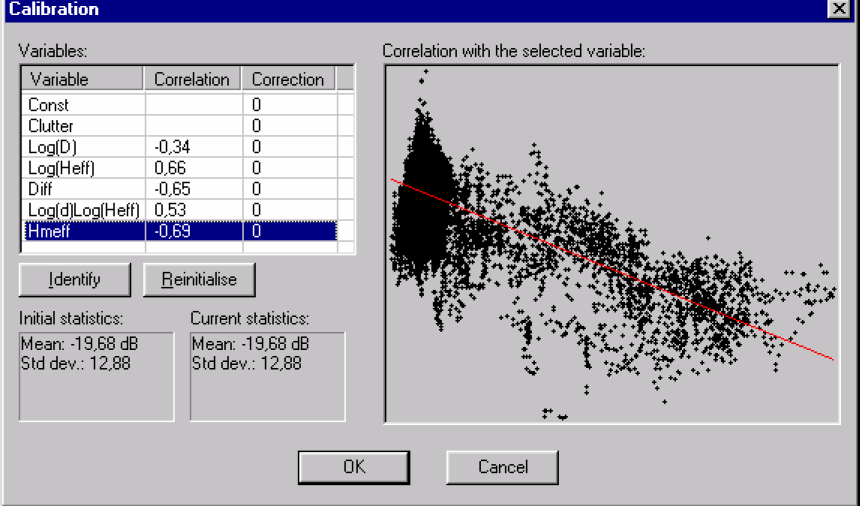
Step#3 Press the calibrate button and find the variable having the highest correlation with error. You can see the regression line when you select this variable.
Step#4 Press Identify, so that Atoll calculates the necessary correction to apply to its related
constant thus decreasing the correlation of this variable with error.
Step#5 Check that the calculated correction does not make the related constant cross the physical limits given below (recommended values).
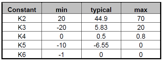
If the constant with the suggested correction respects the given limits, press OK. If the constant with the suggested correction doesn’t respect the given limits, manually set the constant to the limit after pressing Cancel.
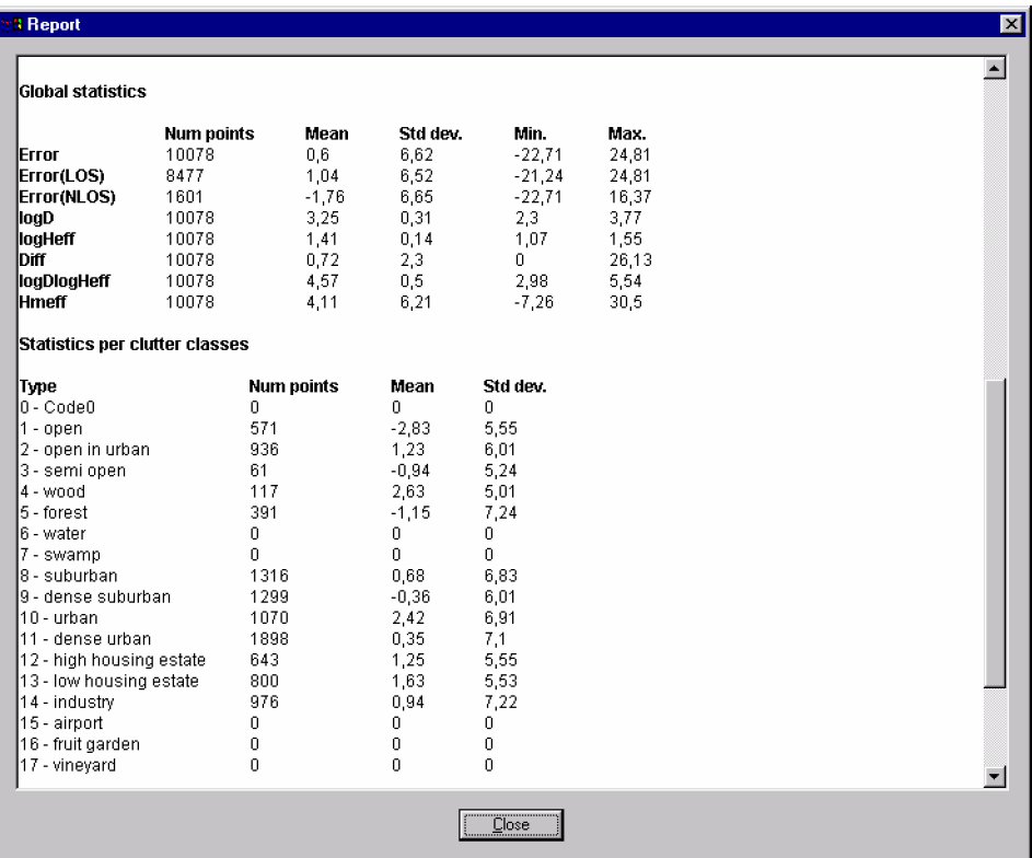
Step#6 You can study the statistics report to check the model accuracy.
Related Posts
- 5G Network RF Planning – Link Budget Basics
- 5G mm Wave 28GHz Band Link Budget-n257
- 5G NR Physical Cell ID (PCI) Planning
- 5G NR Cell Global Identity (NCGI) Planning and Calculations
- 5G NR Network Relationship – Neighbor Planning