Wireless Channel Estimation Using Deep Learning: A Comparison with Least Squares Method

Introduction

In a wireless communication system, transmitted signals experience distortion and attenuation as they propagate through the environment. This effect is usually modelled as a linear time-invariant system with unknown channel parameters. Accurate channel estimation is essential for reliable communication.

Least Square (LS) is a traditional mathematical approach to estimating the channel. This post tries to use Deep Learning (DL) based method that uses neural networks to create a mapping between inputs and outputs.

The LS method computes the analytic solution of the linear equations, while the DL method uses the same data set for 100 epochs to train the neural network.

Experiment Code 

import numpy as np
from tensorflow.keras.models import Sequential
from tensorflow.keras.layers import Dense
import matplotlib.pyplot as plt

n = 1000
p = 5
sigma = 0.1
X = np.random.randn(n, p)
#True Channel
h_true = np.random.randn(p, 1)
y = X.dot(h_true) + sigma * np.random.randn(n, 1)

#LS channel estimation
h_ls, _, _, _ = np.linalg.lstsq(X, y, rcond=None)

#Deep learning model
model = Sequential([
Dense(1, input_dim=p)
])

#Compile the model
model.compile(loss=’mse’, optimizer=’adam’)

#Split data into training and validation sets
val_size = int(0.2 * n)
X_val, y_val = X[:val_size], y[:val_size]
X_train, y_train = X[val_size:], y[val_size:]

#Train model
history = model.fit(X_train, y_train, epochs=100, batch_size=32, validation_data=(X_val, y_val))
h_est = model.get_weights()[0]

print(“True channel parameters: “, h_true.flatten())
print(“Estimated channel parameters using least square method: “, h_ls.flatten())
print(“Estimated channel parameters using deep learning: “, h_est.flatten())

#Plot the results
fig, axs = plt.subplots(nrows=1, ncols=2, figsize=(12, 6))
axs[0].plot(h_true.flatten(), label=”True”)
axs[0].plot(h_ls.flatten(), label=”LS”)
axs[0].plot(h_est, label=”DL”)
axs[0].set_xlabel(“Parameter index”)
axs[0].set_ylabel(“Parameter value”)
axs[0].set_title(“Channel Parameter Estimation”)
axs[0].legend()
axs[1].plot(history.history[‘loss’], label=’Training Loss’)
axs[1].plot(history.history[‘val_loss’], label=’Validation Loss’)
axs[1].set_xlabel(‘Epochs’)
axs[1].set_ylabel(‘Loss’)
axs[1].set_title(‘Training and Validation Loss’)
axs[1].legend()
plt.show()

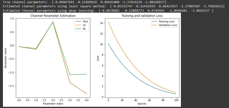
Code Output

The output of the above code is given below. The code plots the true channel parameters, the LS and DL estimates on one subplot, and the training and validation loss on another subplot.

Author

Article Submitted By Mr. Dheeraj Sharma

Related Post

• Smart Antennas and Beamforming, Understanding with GNU : Part 1
• Smart Antennas and Beamforming, Understanding with GNU : Part 2
• Smart Antennas and Beamforming, Understanding with GNU : Part 3